Tutorial 1 - Travel time and carbon emission quantification for car-based trips

Lesson objectives

This tutorial focuses on spatial networks and learn how to construct a routable directed graph for Networkx and find shortest paths along the given street network based on travel times or distance by car. In addition, we will learn how to compute travel-related GHG emissions from car travel.

Introduction to Networkx

In this tutorial we will focus on a network analysis methods that relate to way-finding. Finding a shortest path from A to B using a specific street network is a very common spatial analytics problem that has many practical applications.

Python provides easy to use tools for conducting spatial network analysis. One of the easiest ways to start is to use a library called Networkx which is a Python module that provides a lot tools that can be used to analyze networks on various different ways. It also contains algorithms such as Dijkstra’s algorithm or A* algoritm that are commonly used to find shortest paths along transportation network.

Data and Methodology

In this part, we will learn how to do spatial network analysis in practice.

Typical workflow for routing

If you want to conduct network analysis (in any programming language) there are a few basic steps that typically needs to be done before you can start routing. These steps are:

1. Retrieve data (such as street network from OSM or Digiroad + possibly transit data if routing with PT).

2. Modify the network by adding/calculating edge weights (such as travel times based on speed limit and length of the road segment).

3. Build a routable graph for the routing tool that you are using (e.g. for NetworkX, igraph or OpenTripPlanner).

4. Conduct network analysis (such as shortest path analysis) with the routing tool of your choice.

1. Retrieve data

As a first step, we need to obtain data for routing. Pyrosm library makes it really easy to retrieve routable networks from OpenStreetMap (OSM) with different transport modes (walking, cycling and driving).

• Let’s first extract OSM data for Helsinki that are walkable. In pyrosm, we can use a function called osm.get_network() which retrieves data from OpenStreetMap. It is possible to specify what kind of roads should be retrieved from OSM with network_type -parameter (supports walking, cycling, driving).

from pyrosm import OSM, get_data
import geopandas as gpd
import pandas as pd
import networkx as nx

# Let's read the data that we have previously downloaded from GeoFabrik
osm = OSM("data/Helsinki/Helsinki_larger_region.osm.pbf")

# Parse roads that can be driven by car
roads = osm.get_network(network_type="driving")
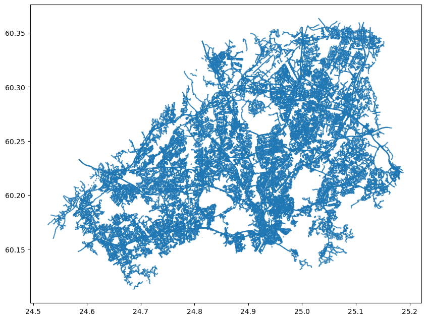
roads.plot(figsize=(10,10))

<Axes: >

roads.head(2)

	access	area	bicycle	bridge	busway	cycleway	est_width	foot	footway	highway	...	tunnel	turn	width	id	timestamp	version	tags	osm_type	geometry	length
0	None	None	None	None	None	None	None	None	None	motorway	...	None	None	None	2293993	1522365641	21	{"visible":false,"light:method":"high_pressure...	way	MULTILINESTRING ((25.12612 60.25746, 25.12709 ...	612.0
1	None	None	no	None	None	None	None	no	None	trunk	...	None	None	None	2294195	1656446984	26	{"visible":false,"TEN-T":"core","functional_cl...	way	MULTILINESTRING ((25.15740 60.23955, 25.15673 ...	144.0

2 rows × 39 columns

Okay, now we have drivable roads as a GeoDataFrame for the city center of Helsinki. If you look at the GeoDataFrame (scroll to the right), we can see that pyrosm has also calculated us the length of each road segment (presented in meters). The geometries are presented here as MultiLineString objects. From the map above we can see that the data also includes short pieces of roads that do not lead to anywhere (i.e. they are isolated). This is a typical issue when working with real-world data such as roads. Hence, at some point we need to take care of those in someway (remove them (typical solution), or connect them to other parts of the network).

In OSM, the information about the allowed direction of movement is stored in column oneway. Let’s take a look what kind of values we have in that column:

roads["oneway"].unique()

array(['yes', None, 'no'], dtype=object)

As we can see the unique values in that column are "yes", "no" or None. We can use this information to construct a directed graph for routing by car. For walking and cycling, you typically want create a bidirectional graph, because the travel is typically allowed in both directions at least in Finland. Notice, that the rules vary by country, e.g. in Copenhagen you have oneway rules also for bikes but typically each road have the possibility to travel both directions (you just need to change the side of the road if you want to make a U-turn). Column maxspeed contains information about the speed limit for given road:

roads["maxspeed"].unique()

array(['100', '70', '80', '60', '40', '30', None, '50', '120', '20', '10',
       '15', '5', 'walk', '25'], dtype=object)

As we can see, there are also None values in the data, meaning that the speed limit has not been tagged for some roads. This is typical, and often you need to fill the non existing speed limits yourself. This can be done by taking advantage of the road class that is always present in column highway:

roads["highway"].unique()

array(['motorway', 'trunk', 'tertiary', 'residential', 'service',
       'secondary', 'unclassified', 'primary', 'cycleway',
       'motorway_link', 'trunk_link', 'primary_link', 'living_street',
       'tertiary_link', 'track', 'secondary_link', 'pedestrian',
       'footway', 'path', 'services', 'steps', 'construction', 'proposed',
       'rest_area'], dtype=object)

Based on these values, we can make assumptions that e.g. residential roads in Helsinki have a speed limit of 30 kmph. Hence, this information can be used to fill the missing values in maxspeed. As we can see, the current version of the pyrosm tool seem to have a bug because some non-drivable roads were also leaked to our network (e.g. footway, cycleway). If you notice these kind of issues with any of the libraries that you use, please notify the developers by raising an Issue in GitHub. This way, you can help improving the software. For this given problem, an issue has already been raised so you don’t need to do it again (it’s always good to check if a related issue exists in GitHub before adding a new one).

Okay, but how can we make a routable graph out of this data of ours? Let’s remind us about the basic elements of a graph that we went through in the lecture slides:

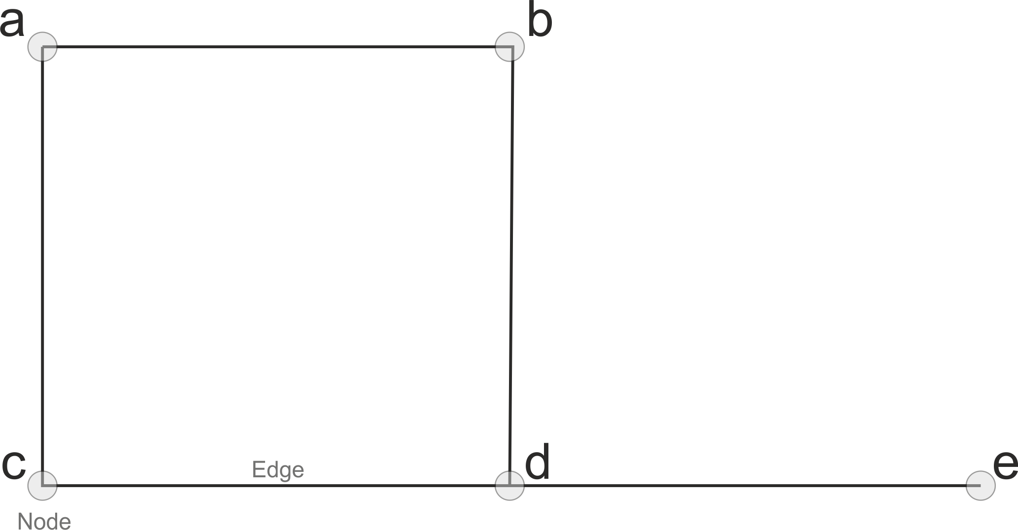
So to be able to create a graph we need to have nodes and edges. Now we have a GeoDataFrame of edges, but where are those nodes? Well they are not yet anywhere, but with pyrosm we can easily retrieve the nodes as well by specifying nodes=True, when parsing the streets:

# Parse nodes and edges
nodes, edges = osm.get_network(network_type="driving", nodes=True)

# Plot the data
ax = edges.plot(figsize=(15,15), color="gray", lw=1.0)
ax = nodes.plot(ax=ax, color="red", markersize=3)

# Zoom in to take a closer look
ax.set_xlim([24.93, 24.945])
ax.set_ylim([60.165, 60.17])

(60.165, 60.17)

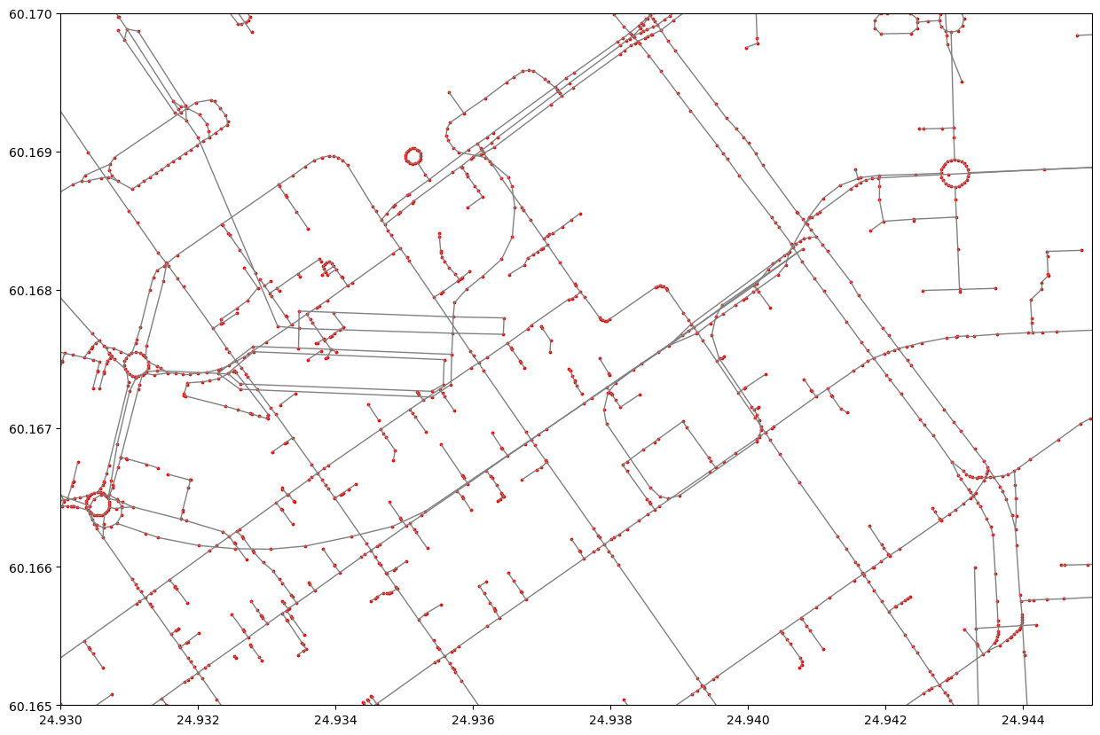
Okay, as we can see now we have both the roads (i.e. edges) and the nodes that connect the street elements together (in red) that are typically intersections. However, we can see that many of the nodes are in locations that are clearly not intersections. This is intented behavior to ensure that we have full connectivity in our network. We can at later stage clean and simplify this network by merging all roads that belong to the same link (i.e. street elements that are between two intersections) which also reduces the size of the network.

Note

In OSM, the street topology is typically not directly suitable for graph traversal due to missing nodes at intersections which means that the roads are not splitted at those locations. The consequence of this, is that it is not possible to make a turn if there is no intersection present in the data structure. Hence, pyrosm will separate all road segments/geometries into individual rows in the data.

Let’s take a look what our nodes data look like:

nodes.head()

	changeset	visible	lon	version	lat	timestamp	tags	id	geometry
0	0	False	25.126116	4	60.257462	0	None	286553	POINT (25.12612 60.25746)
1	0	False	25.127092	1	60.257626	0	None	1393097609	POINT (25.12709 60.25763)
2	0	False	25.127998	2	60.257771	0	None	766312702	POINT (25.12800 60.25777)
3	0	False	25.129299	1	60.257961	0	None	1393097450	POINT (25.12930 60.25796)
4	0	False	25.129543	1	60.257996	0	None	4118526050	POINT (25.12954 60.25800)

As we can see, the nodes GeoDataFrame contains information about the coordinates of each node as well as a unique id for each node. These id values are used to determine the connectivity in our network. Hence, pyrosm has also added two columns to the edges GeoDataFrame that specify from and to ids for each edge. Column u contains information about the from-id and column v about the to-id accordingly:

# Check last four columns
edges.iloc[:5,-4:]

	geometry	u	v	length
0	LINESTRING (25.12612 60.25746, 25.12709 60.25763)	286553	1393097609	56.875
1	LINESTRING (25.12709 60.25763, 25.12800 60.25777)	1393097609	766312702	52.513
2	LINESTRING (25.12800 60.25777, 25.12930 60.25796)	766312702	1393097450	74.826
3	LINESTRING (25.12930 60.25796, 25.12954 60.25800)	1393097450	4118526050	13.998
4	LINESTRING (25.12954 60.25800, 25.13060 60.25814)	4118526050	766312444	60.794

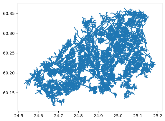
We can see that the geometries are now stored as LineString instead of MultiLineString. At this point, we can fix the issue related to having some pedestrian roads in our network. We can do this by removing all edges from out GeoDataFrame that have highway value in 'cycleway', 'footway', 'pedestrian', 'trail', 'crossing':

edges = edges.loc[~edges["highway"].isin(['cycleway', 'footway', 'pedestrian', 'trail', 'crossing'])].copy()
edges.plot()

<Axes: >

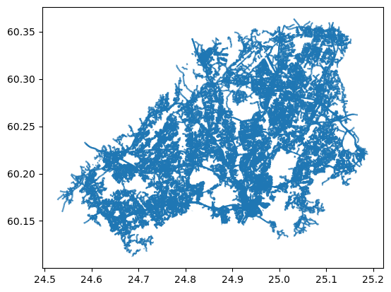
Now we can see, that some of the isolated edges were removed from the data. The character ~ (tilde) in the command above is a negation operator that is handy if you want to e.g. remove some rows from your GeoDataFrame based on criteria such as we used here.

2. Modify the data

At this stage, we have the necessary components to build a routable graph (nodes and edges) based on distance. However, in real life the network distance is not the best cost metric to use, because the shortest path (based on distance) is not necessarily always the optimal route in terms of travel time. Time is typically the measure that people value more (plus it is easier to comprehend), so at this stage we want to add a new cost attribute to our edges GeoDataFrame that converts the metric distance information to travel time (in seconds) based on following formula:

• <distance-in-meters> / (<speed-limit-kmph> / 3.6)

Before we can do this calculation, we need to ensure that all rows in maxspeed column have information about the speed limit. Let’s check the value counts of the column and also include information about the NaN values with dropna parameter:

# Count values
edges["maxspeed"].value_counts(dropna=False)

maxspeed
None    229362
30       89066
40       52048
50       25098
80        8283
60        5123
20        4365
100       1700
10         830
70         551
120        467
15         199
5           38
walk        16
25           9
Name: count, dtype: int64

As we can see, the rows which do not contain information about the speed limit is the second largest group in our data. Hence, we need to apply a criteria to fill these gaps. We can do this based on following “rule of thumb” criteria in Finland (notice that these vary country by country):

Road class	Speed limit within urban region	Speed limit outside urban region
motorway	100	120
motorway_link	80	80
trunk	60	100
trunk_link	60	60
primary	50	80
primary_link	50	50
secondary	50	50
secondary_link	50	50
tertiary	50	60
tertiary_link	50	50
unclassified	50	80
unclassified_link	50	50
residential	50	80
living_street	20	NA
service	30	NA
other	50	80

For simplicity, we can consider that all the roads in Helsinki Region follows the within urban region speed limits, although this is not exactly true (the higher speed limits start somewhere at the outer parts of the city region). For making the speed limit values more robust / correct, you could use data about urban/rural classification which is available in Finland from Finnish Environment Institute. Let’s first convert our maxspeed values to integers using astype() method:

edges = edges[edges.maxspeed != 'walk']
edges["maxspeed"] = edges["maxspeed"].astype(float).astype(pd.Int64Dtype())
edges["maxspeed"].unique()

/opt/miniconda3/envs/geo/lib/python3.11/site-packages/geopandas/geodataframe.py:1528: SettingWithCopyWarning: 
A value is trying to be set on a copy of a slice from a DataFrame.
Try using .loc[row_indexer,col_indexer] = value instead

See the caveats in the documentation: https://pandas.pydata.org/pandas-docs/stable/user_guide/indexing.html#returning-a-view-versus-a-copy
  super().__setitem__(key, value)

<IntegerArray>
[100, 70, 80, 60, 40, 30, <NA>, 50, 120, 20, 10, 15, 5, 25]
Length: 14, dtype: Int64

As we can see, now the maxspeed values are stored in integer format inside an IntegerArray, and the None values were converted into pandas.NA objects that are assigned with <NA>. Now we can create a function that returns a numeric value for different road classes based on the criteria in the table above:

def road_class_to_kmph(road_class):
    """
    Returns a speed limit value based on road class, 
    using typical Finnish speed limit values within urban regions.
    """
    if road_class == "motorway":
        return 100
    elif road_class == "motorway_link":
        return 80
    elif road_class in ["trunk", "trunk_link"]:
        return 60
    elif road_class == "service":
        return 30
    elif road_class == "living_street":
        return 20
    else:
        return 50

Now we can apply this function to all rows that do not have speed limit information:

# Separate rows with / without speed limit information 
mask = edges["maxspeed"].isnull()
edges_without_maxspeed = edges.loc[mask].copy()
edges_with_maxspeed = edges.loc[~mask].copy()

# Apply the function and update the maxspeed
edges_without_maxspeed["maxspeed"] = edges_without_maxspeed["highway"].apply(road_class_to_kmph)
edges_without_maxspeed.head(5).loc[:, ["maxspeed", "highway"]]

	maxspeed	highway
34	30	service
35	30	service
36	30	service
37	30	service
38	30	service

Okay, as we can see now the maxspeed value have been updated according our criteria, and e.g. the service road class have been given the speed limit 30 kmph. Now we can recreate the edges GeoDataFrame by combining the two frames:

edges = pd.concat([edges_with_maxspeed, edges_without_maxspeed])
edges.head(-10).loc[:, ["maxspeed", "highway"]]
edges["maxspeed"].unique()

<IntegerArray>
[100, 70, 80, 60, 40, 30, 50, 120, 20, 10, 15, 5, 25]
Length: 13, dtype: Int64

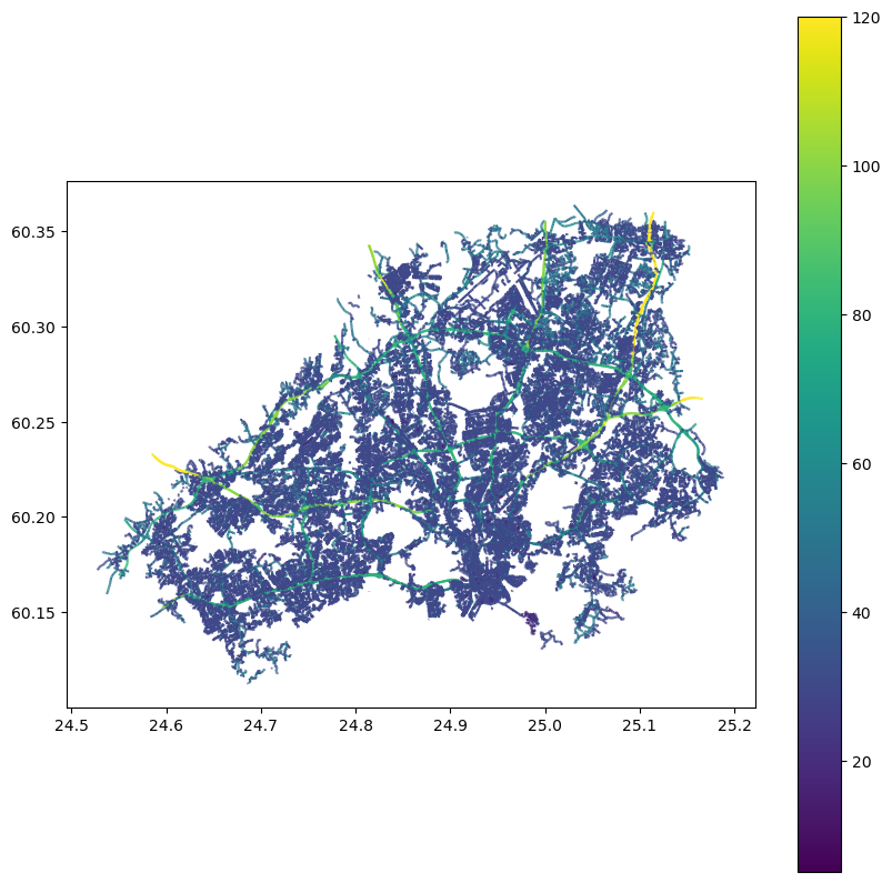
Great, now all of our edges have information about the speed limit. We can also visualize them:

# Convert the value into regular integer Series (the plotting requires having Series instead of IntegerArray) 
edges["maxspeed"] = edges["maxspeed"].astype(int)
ax = edges.plot(column="maxspeed", figsize=(10,10), legend=True)

Finally, we can calculate the travel time in seconds using the formula we saw earlier and add that as a new cost attribute for our network:

edges["travel_time_seconds"] = edges["length"] / (edges["maxspeed"]/3.6)
edges.iloc[0:10, -4:]

	u	v	length	travel_time_seconds
0	286553	1393097609	56.875	2.047500
1	1393097609	766312702	52.513	1.890468
2	766312702	1393097450	74.826	2.693736
3	1393097450	4118526050	13.998	0.503928
4	4118526050	766312444	60.794	2.188584
5	766312444	5515330945	82.557	2.972052
6	5515330945	286537	16.953	0.610308
7	286537	1393097550	78.388	2.821968
8	1393097550	286536	174.982	6.299352
9	251606513	1133480099	54.846	2.820651

Excellent! Now our GeoDataFrame has all the information we need for creating a graph that can be used to conduct shortest path analysis based on length or travel time. Notice that here we assume that the cars can drive with the same speed as what the speed limit is. Considering the urban dynamics and traffic congestion, this assumption might not hold, but for simplicity, we assume so in this tutorial.

3. Build a directed graph for routing using pyrosm

Now as we have calculated the travel time for our edges. We still need to convert our nodes and edges into a directed graph, so that we can start using it for routing. There are easy-to-use functionalities for doing this in pyrosm and osmnx.

As a background information, it is good to understand that our edges represents a directed network. This means that the information stored in oneway column will be used to determine the network structure for the edges based on the rules in that column. If the oneway is 'yes', it means that the street can be driven only to one direction, and if it is None or has a value "no", then that road can be driven to both directions. This means that the tool will make new duplicate edge and reversing the from-id and to-id values in the u and v columns in the data. In addition, value -1 in the oneway column means that the road can only be driven to one direction but against the digitization direction. In such cases, the edge is flipped: the to-id (u) and from-id (u) is reversed so that the directionality in the graph is correctly specified.

• Let’s see how we can create a routable NetworkX graph using pyrosm with one command:

G = osm.to_graph(nodes, edges, graph_type="networkx")
G

<networkx.classes.multidigraph.MultiDiGraph at 0x310cbd110>

Now we have a routable graph. pyrosm actually does some additional steps in the background. By default, pyrosm cleans all unconnected edges from the graph and only keeps edges that can be reached from every part of the network. In addition, pyrosm automatically modifies the graph attribute information in a way that they are compatible with OSMnx that provides many handy functionalities to work with graphs. Such as converting the graph into a GeoDataFrame which we can then plot normally using .plot():

import osmnx as ox 

# Convert the graph edges to GeoDataFrame
edges_gdf = ox.graph_to_gdfs(G, nodes=False)

# Plot
edges_gdf.plot()

<Axes: >

4. Routing with NetworkX

Now we have everything we need to start routing with NetworkX (based on driving distance or travel time). But first, let’s again go through some basics about routing.

Basic logic in routing

Most (if not all) routing algorithms work more or less in a similar manner. The basic steps for finding an optimal route from A to B, is to:

1. Find the nearest node for origin location * (+ get info about its node-id and distance between origin and node)

2. Find the nearest node for destination location * (+ get info about its node-id and distance between origin and node)

3. Use a routing algorithm to find the shortest path between A and B

4. Retrieve edge attributes for the given route(s) and summarize them (can be distance, time, CO2, or whatever)

* in more advanced implementations you might search for the closest edge

This same logic should be applied always when searching for an optimal route between a single origin to a single destination, or when calculating one-to-many -type of routing queries (producing e.g. travel time matrices).

Find the optimal route between two locations

Next, we will learn how to find the shortest path between two locations using Dijkstra’s algorithm.

We use the following coodrinates as our origin and destinations for demonstration purposes.

# OSM data is in WGS84 so typically we need to use lat/lon coordinates when searching for the closest node

# Origin

orig_y, orig_x = 60.16874416, 24.95721918  # notice the coordinate order (lon, lat)!

# Destination

dest_y, dest_x =  60.1622494, 24.9082137 ##60.16872763, 24.92119326

print("Origin coords:", orig_x, orig_y)
print("Destination coords:", dest_x, dest_y)

Origin coords: 24.95721918 60.16874416
Destination coords: 24.9082137 60.1622494

Okay, we have coordinates now for our origin and destination. Let us find the closest osm nodes for the selected origin and destination locations in the area.

Find the nearest nodes

Next, we need to find the closest nodes from the graph for both of our locations. For calculating the closest point we use ox.distance.nearest_nodes() -function and specify return_dist=True to get the distance in meters.

# 1. Find the closest nodes for origin and destination
orig_node_id, dist_to_orig = ox.distance.nearest_nodes(G, X=orig_x, Y=orig_y, return_dist=True)
dest_node_id, dist_to_dest = ox.distance.nearest_nodes(G, X=dest_x, Y=dest_y, return_dist=True)

print("Origin node-id:", orig_node_id, "and distance:", dist_to_orig, "meters.")
print("Destination node-id:", dest_node_id, "and distance:", dist_to_dest, "meters.")

Origin node-id: 1015191942 and distance: 17.151166613537725 meters.
Destination node-id: 299272103 and distance: 4.266050236105179 meters.

Now we are ready to start the actual routing with NetworkX.

Find the fastest route by distance / time

Now we can do the routing and find the shortest path between the origin and target locations by using the dijkstra_path() function of NetworkX. For getting only the cumulative cost of the trip, we can directly use a function dijkstra_path_length() that returns the travel time without the actual path.

With weight -parameter we can specify the attribute that we want to use as cost/impedance. We have now three possible weight attributes available: 'length' and 'travel_time_seconds'.

• Let’s first calculate the routes between locations by walking and cycling, and also retrieve the travel times

# Calculate the paths by walking and cycling
metric_path = nx.dijkstra_path(G, source=orig_node_id, target=dest_node_id, weight='length')
time_path = nx.dijkstra_path(G, source=orig_node_id, target=dest_node_id, weight='travel_time_seconds')

# Get also the actual travel times (summarize)
travel_length = nx.dijkstra_path_length(G, source=orig_node_id, target=dest_node_id, weight='length')
travel_time = nx.dijkstra_path_length(G, source=orig_node_id, target=dest_node_id, weight='travel_time_seconds')

Okay, that was it! Let’s now see what we got as results by visualizing the results.

For visualization purposes, we can use a handy function again from OSMnx called ox.plot_graph_route() (for static) or ox.plot_route_folium() (for interactive plot).

• Let’s first make static maps

# Shortest path based on distance
fig, ax = ox.plot_graph_route(G, metric_path)

# Add the travel time as title
ax.set_xlabel("Shortest path distance {t: .1f} meters.".format(t=travel_length))

Text(0.5, 133.03826062620507, 'Shortest path distance  3277.5 meters.')

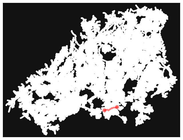
fig, ax = ox.plot_graph_route(G, time_path)

# Add the travel time as title
ax.set_xlabel("Travel time {t: .1f} minutes.".format(t=travel_time/60))

Text(0.5, 133.03826062620507, 'Travel time  5.7 minutes.')

Great! Now we have successfully found the optimal route between our origin and destination and we also have estimates about the travel time that it takes to travel between the locations by walking and cycling. As we can see, the route for both travel modes is exactly the same which is natural, as the only thing that changed here was the constant travel speed.

• Let’s still finally see an example how you can plot a nice interactive map out of our results with OSMnx:

# Notice: The following requires an internet connection
ox.plot_route_folium(G, time_path, popup_attribute='travel_time_seconds')

/var/folders/f7/rhmqxfmx40s4yv9bhh7skq4m0000gp/T/ipykernel_74524/1260170060.py:1: FutureWarning: The `folium` module has been deprecated and will be removed in the v2.0.0 release. You can generate and explore interactive web maps of graph nodes, edges, and/or routes automatically using GeoPandas.GeoDataFrame.explore instead, for example like: `ox.graph_to_gdfs(G, nodes=False).explore()`. See the OSMnx examples gallery for complete details and demonstrations.
  ox.plot_route_folium(G, time_path, popup_attribute='travel_time_seconds')

Make this Notebook Trusted to load map: File -> Trust Notebook

# Calculate and return the path length directly
time_path_distance = nx.path_weight(G, time_path, weight='length')
print(f"The travel distance: {time_path_distance:.0f} meters")

The travel distance: 3299 meters

Load the GHG emission data for Car travel

Here we calculate the carbon emission factors for the single OD pair. Let us now import the GHG emissions per passenger-kilometer (g CO₂/pkm) by transport modes Data from the file “LCA_gCO2_per_pkm_by_transport_mode.csv”.

The explanations of the acronyms (in the transport modes names) are: BEV = battery electric vehicle; HEV = hybrid electric vehicle; ICE = internal combustion engine; FCEV = fuel cell electric vehicle; PHEV = plug-in hybrid electric vehicle.

#import pandas as pd
ghg_pkm_pv = pd.read_csv("data/LCA_gCO2_per_pkm_by_transport_mode.csv",index_col=0)
ghg_pkm_pv.loc['Total_gCO2'] = ghg_pkm_pv.sum(axis=0)
ghg_pkm_pv.head()

	Private e-scooter	Shared e-scooter (1st gen.)	Shared e-scooter (new gen.)	Private bike	Shared bike	Private e-bike	Shared e-bike	Private moped - ICE	Private moped - BEV	Shared moped - ICE	...	Ridesourcing - car - PHEV	Ridesourcing - car - BEV	Ridesourcing - car - BEV (two packs)	Ridesourcing - car - FCEV	Bus - ICE	Bus - HEV	Bus - BEV	Bus - BEV (two packs)	Bus - FCEV	Metro/urban train
Vehicle component	26	71	66	7	23	13	37	8	10	20	...	29	39	62	32	8	8	14	17	11	2
Fuel component	1	1	2	0	0	3	3	54	5	54	...	64	16	16	80	72	53	10	10	44	12
Infrastructure componen	9	9	9	9	9	9	10	11	11	11	...	21	20	20	21	4	4	4	4	4	11
Operational services	0	35	25	0	25	0	25	0	0	0	...	59	15	15	73	8	6	1	1	5	0
Total_gCO2	36	116	102	16	57	25	75	73	26	85	...	173	90	113	206	92	71	29	32	64	25

5 rows × 32 columns

# Emissions for different types of cars
Car_related_transit_modes = ['Private car - ICE', 'Private car - HEV', 'Private car - PHEV',
       'Private car - BEV', 'Private car - FCEV', 'Taxi - HEV', 'Taxi - BEV',
       'Taxi - BEV (two packs)', 'Taxi - FCEV']

# For the sake of simplicity, calculate the emissions based on an average out of all types 
# (alternatively you could also pick values for specific type of vehicle)
avg_CO2_emission_Car = ghg_pkm_pv.loc['Total_gCO2', Car_related_transit_modes].mean()
avg_CO2_emission_Car

155.44444444444446

Now we can see that the average CO2 emission per kilometer is 155 grams per passenger kilometer. To calculate the emissions of the trip that we computer earlier, we can do a simple mathematical calculation:

# Calculate the emissions for the single trip
emissions = avg_CO2_emission_Car * time_path_distance / 1000
print(f"Carbon emissions of the trip: {emissions:.0f} grams.")

Carbon emissions of the trip: 513 grams.