Introduction to Data

Getting started

There are basically three options to run the codes in this tutorial:

1. Copy-Paste the codes from the website and run the codes line-by-line on your own computer with your preferred IDE (Jupyter Lab, Spyder, PyCharm etc.).

2. Download this Notebook (see below) and run it using Jupyter Lab which you should have installed by following the installation instructions.

3. Run the codes using Binder (see below) which is the easiest way, but has very limited computational resources (i.e. can be very slow).

Download the Notebook

You can download this tutorial Notebook to your own computer by clicking the Download button from the Menu on the top-right section of the website.

• Right-click the option that says .ipynb and choose “Save link as ..”

Run the codes on your own computer

Before you can run this Notebook, and/or do any programming, you need to launch the Jupyter Lab programming environment. The JupyterLab comes with the environment that you installed earlier (if you have not done this yet, follow the installation instructions). To run the JupyterLab:

1. Using terminal/command prompt, navigate to the folder where you have downloaded the Jupyter Notebook tutorial: $ cd /mydirectory/

2. Activate the programming environment: $ conda activate geo

3. Launch the JupyterLab: $ jupyter lab

After these steps, the JupyterLab interface should open, and you can start executing cells (see hints below at “Working with Jupyter Notebooks”).

Alternatively: Run codes in Binder (with limited resources)

Alternatively (not recommended due to limited computational resources), you can run this Notebook by launching a Binder instance. You can find buttons for activating the python environment at the top-right of this page which look like this:

Working with Jupyter Notebooks

Jupyter Notebooks are documents that can be used and run inside the JupyterLab programming environment containing the computer code and rich text elements (such as text, figures, tables, and links).

A couple of hints:

• You can execute a cell by clicking a given cell that you want to run and pressing Shift + Enter (or by clicking the “Play” button on top)

• You can change the cell-type between Markdown (for writing text) and Code (for writing/executing code) from the dropdown menu above.

See further details and help for using Notebooks and JupyterLab from here.

Lesson objectives

This tutorial focuses on how to work with various geospatial data to construct a spatial networks and learn how to construct a routable directed graph for Networkx and find shortest paths along the given street network based on travel times or distance by car using R5py. In addition, we will learn about the relevant data to calculate GHG emissions for different travel modes of commutating among multiple origin-destination zones simultaneously.

Data requirements

Data for creating a routable network

R5py is a Python library for routing and calculating travel time matrices on multimodal transport networks (walk, bike, public transport and car). It provides a simple and friendly interface to R⁵ (the Rapid Realistic Routing on Real-world and Reimagined networks) which is a routing engine developed by Conveyal. R5py is designed to interact with GeoPandas GeoDataFrames, and it is inspired by r5r which is a similar wrapper developed for R. R5py exposes some of R5’s functionality via its Python API, in a syntax similar to r5r’s. At the time of this writing, only the computation of travel time matrices has been fully implemented. Over time, r5py will be expanded to incorporate other functionalities from R5. When calculating travel times with r5py, you typically need a couple of datasets:

• A road network dataset from OpenStreetMap (OSM) in Protocolbuffer Binary (.pbf) -format:

  • This data is used for finding the fastest routes and calculating the travel times based on walking, cycling and driving. In addition, this data is used for walking/cycling legs between stops when routing with transit.

  • Hint: Sometimes you might need modify the OSM data beforehand, e.g. by cropping the data or adding special costs for travelling (e.g. for considering slope when cycling/walking). When doing this, you should follow the instructions at Conveyal website. For adding customized costs for pedestrian and cycling analyses, see this repository.

• A transit schedule dataset in General Transit Feed Specification (GTFS.zip) -format (optional):

  • This data contains all the necessary information for calculating travel times based on public transport, such as stops, routes, trips and the schedules when the vehicles are passing a specific stop. You can read about GTFS standard from here.

  • Hint: r5py can also combine multiple GTFS files, as sometimes you might have different GTFS feeds representing e.g. the bus and metro connections.

Where to get these datasets?

Here are a few places from where you can download the datasets for creating the routable network:

• OpenStreetMap data in PBF-format:

  • pyrosm -library. Allows downloading data directly from Python (based on GeoFabrik and BBBike).

  • pydriosm -library. Allows downloading data directly from Python (based on GeoFabrik and BBBike).

  • GeoFabrik -website. Has data extracts for many pre-defined areas (countries, regions, etc).

  • BBBike -website. Has data extracts readily available for many cities across the world. Also supports downloading data by specifying your own area or interest.

  • Protomaps -website. Allows to download the data with custom extent by specifying your own area of interest.

• GTFS data:

  • Transitfeeds -website. Easy to navigate and find GTFS data for different countries and cities. Includes current and historical GTFS data. Notice: The site will be depracated in the future.

  • Mobility Database -website. Will eventually replace TransitFeeds -website.

  • Transitland -website. Find data based on country, operator or feed name. Includes current and historical GTFS data.

Data for origin and destination locations (H3 hexagonal grid)

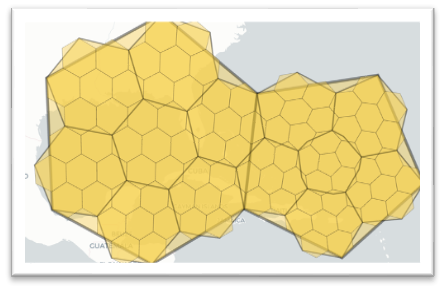
In addition to OSM and GTFS datasets, you need data that represents the origin and destination locations (OD-data) for routings and understanding the number of people travelling between them. This data is typically stored in one of the geospatial data formats, such as Shapefile, GeoJSON or GeoPackage. In the workshop tutorials, we are using H3 hexagonal grid data at resolution 9 to represent the origin-destination locations (scroll down for further details with code):

Travel demand: Mobile Phone Data

To understand the travel demand in a given city (i.e. how many people travel between given locations), you need to have some data that is able to provide that information. Traditionally travel surveys and statistics have been used for this purpose, but in this workshop we are using mobile phone data from a company called Locomizer to extract information about the travel demand in Helsinki Region. Locomizer data is aggregated and anonymized into H3 hexagons and it reveals the number of users that travel from a given origin hexagon to a given destination hexagon at a specific day and hour (i.e. revealing Origin-destination flows in the city).

In this tutorial, we share you aggregated mobility data that represents the OD-flows in Helsinki Region at H9-resolution during a regular Thursday recorded between April 15th to May 15th 2023:

Data for GHG emission factors

The International Transport Forum (ITF) has developed a comprehensive life-cycle analysis Excel-based tool of urban transport modes including new mobility services, such as shared vehicles and ridesourcing. The Excel-based tool (provide the link?) includes calculations and assumptions made for the ITF report titled as “Good to go? Assessing the environmental performance of new mobility in cities”.

• Sources:

  • Cazzola, P. and Crist, P., 2020. Good to go? Assessing the environmental performance of new mobility

  • The electricity generation mix of Finland in 2020.

From these sources, a CSV file named “LCA_gCO2_per_pkm_by_transport_mode.csv” is created, consisting of GHG emissions per passenger-kilometer (g CO₂/pkm) by transport modes derived from the mentioned LCA tool by ITF. The columns represent the different transport modes and the rows represent the GHG emissions. The GHG emissions of the transport modes have been divided into four separate components: vehicle component, fuel component, infrastructure component and operational services. The explanations of the acronyms (in the transport modes names) are: BEV = battery electric vehicle; HEV = hybrid electric vehicle; ICE = internal combustion engine; FCEV = fuel cell electric vehicle; PHEV = plug-in hybrid electric vehicle.

Helsinki Regional Transport Authority (HSL) survey data

The Helsinki Regional Transport Authority (Finnish: Helsingin seudun liikenne, HSL; Swedish: Helsingforsregionens trafik, HRT) is the inter-municipal body responsible for maintaining the public transportation network across the nine municipalities of Greater Helsinki, Finland.

HSL oversees the operation of Helsinki’s entire public transportation system, which includes local buses, trams, metro trains, ferries, commuter trains, and bikeshare services. According to an HSL survey on the number of trips, residents of the Helsinki region aged seven and above made a total of 4.6 million trips on a typical weekday in the fall of 2023. The detailed report can be found here.

Based on the modality of travel choice and different percentages of various weekday trips of residents of the Helsinki region in autumn 2023, the survey report contains the following ratio of travel mode share in the HSL-alue yhteensä (i.e. total HSL area):

Car_share_Hsl = 0.35 ## Car
PT_share_Hsl = 0.23 ## Public transport
Bike_share_Hsl = 0.08  ## Bicycle
Walk_share_Hsl = 0.33  ## Walking
Other_share_Hsl = 0.01 ## Other

This data can be used to split the travellers among OD hexagon pairs accordingly to calculate more representative CO2 emissions for given origin-destination pairs.

Introduction to H3 Hexagonal Hierarchical Geospatial Indexing System

In this tutorial, first, we will learn how to work with Uber’s H3 Hexagonal Hierarchical Geospatial Indexing System in Python. We will utilize the geographical data around the city center area of Helsinki, Finland.

# A point of interest (poi) at the Helsinki Central Location
from shapely.geometry import Point 
import osmnx as ox
import geopandas as gpd

# Geocode a specific place in Helsinki
address = "Scandic Hub, Helsinki" 
lat, lon = ox.geocode(address)

# Create a GeoDataFrame out of the coordinates
poi = gpd.GeoDataFrame({"geometry": [Point(lon, lat)], "name": "Scandic Hub, Helsinki", "id": [0]}, index=[0], crs="epsg:4326")
# plotting the poi
poi.explore(max_zoom=13, color="red", marker_kwds={"radius": 12})

Make this Notebook Trusted to load map: File -> Trust Notebook

We can select a set of neighbouring hexagon cells of resolution 9 from the centre of Helsinki. This can be achieved by the following function. Details can be found here. The syntaxes used in this tutorial work for the h3 version v3.7.7.

import shapely
import h3
import matplotlib.pyplot as plt

# h3 hexagons are to be created at a specified resolution from 1-10 
resolution = 9

# We can indicate the number of hexagonal rings around the central hexagon
ring_size = 6

# Get the H3 hexagons covering the central Helsinki 
center_h3 = h3.geo_to_h3(lat, lon, resolution) 
hexagons = list(h3.k_ring(center_h3, ring_size))  # Convert the set to a list

# Create a GeoDataFrame with hexagons and their corresponding geometries
hexagon_geometries = [shapely.geometry.Polygon(h3.h3_to_geo_boundary(hexagon, geo_json=True)) for hexagon in hexagons]
hexagon_df = gpd.GeoDataFrame({'Hexagon_ID': hexagons, 'geometry': hexagon_geometries},crs="epsg:4326")
#hexagon_df.explore()

## Create a column of centroids and make them as point geometry
hexagon_df["H3_centroids"] = hexagon_df.Hexagon_ID.apply(lambda x: Point(h3.h3_to_geo(str(x))))
hexagon_df.head()

	Hexagon_ID	geometry	H3_centroids
0	891126d3397ffff	POLYGON ((24.92704 60.17126, 24.92973 60.17057...	POINT (60.17227604844199 24.929499715958208)
1	891126d322fffff	POLYGON ((24.94227 60.15421, 24.94496 60.15352...	POINT (60.15521837639684 24.944728818026114)
2	891126d32a3ffff	POLYGON ((24.92396 60.15563, 24.92664 60.15494...	POINT (60.156642821084354 24.926409550192375)
3	891126d14a7ffff	POLYGON ((24.96215 60.16060, 24.96483 60.15991...	POINT (60.16160881879764 24.964603523430327)
4	891126d3357ffff	POLYGON ((24.94382 60.16202, 24.94650 60.16133...	POINT (60.163035534643534 24.946277954619735)

Load and prepare the origin and destination data

We will use a pair of these hexagons as origin and destinations to understand the travel patterns of commuters and Green House Gas (GHG) emissions of individual users due to different modes of transport. For this tutorial, we will use a sample of H3 hexagons that correspond with the Locomizer data at resolution 9 in the Helsinki region.

Reading the Locomizer data

Let’s start by understanding a sample of the Locomizer dataset into a pandas DataFrame that we can use as origin-destination hexagons that contain the number of users travelled in between.

import pandas as pd
import shapely

# Reading the OD data
data = pd.read_csv("data/Locomizer_data/Locomizer_Valid_OD_Hexes_filtered.csv",index_col=0)

data.head()

	destination_code_level_9	origin_code_level_9	NUMBER_OF_USERS	DWELL_TIME	EXTRAPOLATED_NUMBER_OF_USERS	NUMBER_OF_SIGNALS	EXTRAPOLATED_NUMBER_OF_SIGNALS	PROPORTION_OF_USERS	NAMEFIN
0	890899695b3ffff	89089961267ffff	0.666667	5.487959	92.888889	7.444444	935.555556	5.026455	Helsinki
1	8908996800bffff	89089968003ffff	3.666667	3.687860	362.555556	5.222222	509.666667	9.801587	Helsinki
2	8908996800fffff	89089968003ffff	0.666667	2.012012	71.000000	0.888889	92.222222	1.014911	Helsinki
3	8908996801bffff	89089968003ffff	0.666667	2.665467	79.111111	1.222222	154.111111	4.021164	Helsinki
4	89089968063ffff	89089968003ffff	2.000000	3.959179	235.666667	2.555556	287.888889	4.082492	Helsinki

The loco_sample_OD DataFrame contains a few columns, namely origin_code_level_9, destination_code_level_9, DAY NUMBER_OF_USERS, DWELL_TIME, EXTRAPOLATED_NUMBER_OF_USERS NUMBER_OF_SIGNALS, EXTRAPOLATED_NUMBER_OF_SIGNALS, PROPORTION_OF_USERS, and NAMEFIN. We will begin with visualising origin hexagons with valid users in H3 hexagonal resolution 9. As we can see, there is no geometry column with the unique boundary values of the hexagons. The origin and destination hexagon geometry columns are required for defining the hexagonal boundaries to work.

Hence, we have to create the hexagonal geometries as below:

# Name of the hex code column that we want to use for creating geometries
hex_col = "destination_code_level_9"

# Create geometries
data["geometry"] = data[hex_col].apply(lambda x: shapely.Polygon(h3.h3_to_geo_boundary(x, geo_json=True))) 

data.head()

	destination_code_level_9	origin_code_level_9	NUMBER_OF_USERS	DWELL_TIME	EXTRAPOLATED_NUMBER_OF_USERS	NUMBER_OF_SIGNALS	EXTRAPOLATED_NUMBER_OF_SIGNALS	PROPORTION_OF_USERS	NAMEFIN	geometry
0	890899695b3ffff	89089961267ffff	0.666667	5.487959	92.888889	7.444444	935.555556	5.026455	Helsinki	POLYGON ((24.718877380241732 60.16058820239154...
1	8908996800bffff	89089968003ffff	3.666667	3.687860	362.555556	5.222222	509.666667	9.801587	Helsinki	POLYGON ((24.72557001608462 60.18673401028163,...
2	8908996800fffff	89089968003ffff	0.666667	2.012012	71.000000	0.888889	92.222222	1.014911	Helsinki	POLYGON ((24.727778540207243 60.18944780076118...
3	8908996801bffff	89089968003ffff	0.666667	2.665467	79.111111	1.222222	154.111111	4.021164	Helsinki	POLYGON ((24.72044178952002 60.186403225409265...
4	89089968063ffff	89089968003ffff	2.000000	3.959179	235.666667	2.555556	287.888889	4.082492	Helsinki	POLYGON ((24.735827572834758 60.18739503712752...

To better understand the mobility patterns in the region, let’s aggregate the movement flows and create a map that shows the number of users in the destination cells:

# Aggregate the OD-flows and show how many people travel to specific destinations
pop_dest = data.groupby(hex_col)["EXTRAPOLATED_NUMBER_OF_USERS"].sum().reset_index()
pop_dest.head()

	destination_code_level_9	EXTRAPOLATED_NUMBER_OF_USERS
0	890899612cbffff	352.444444
1	89089968003ffff	181.222222
2	8908996800bffff	1051.666667
3	8908996800fffff	71.000000
4	8908996801bffff	79.111111

Now we know how many users have travelled to specific destination. Next, we will create geometries (again) and turn these into a GeoDataFrame based on the H3 codes:

pop_dest["geometry"] = pop_dest[hex_col].apply(lambda x: shapely.Polygon(h3.h3_to_geo_boundary(x, geo_json=True)))
pop_dest = gpd.GeoDataFrame(pop_dest, crs="epsg:4326")

pop_dest.head()

	destination_code_level_9	EXTRAPOLATED_NUMBER_OF_USERS	geometry
0	890899612cbffff	352.444444	POLYGON ((24.61873 60.22864, 24.62142 60.22796...
1	89089968003ffff	181.222222	POLYGON ((24.72265 60.18912, 24.72533 60.18843...
2	8908996800bffff	1051.666667	POLYGON ((24.72557 60.18673, 24.72825 60.18605...
3	8908996800fffff	71.000000	POLYGON ((24.72778 60.18945, 24.73046 60.18876...
4	8908996801bffff	79.111111	POLYGON ((24.72044 60.18640, 24.72312 60.18572...

Finally, we can visualize the number of users at specific destination cells:

# Visualize destination 
pop_dest.plot(column="EXTRAPOLATED_NUMBER_OF_USERS", cmap="Reds", legend=True, figsize=(12,8))

<Axes: >

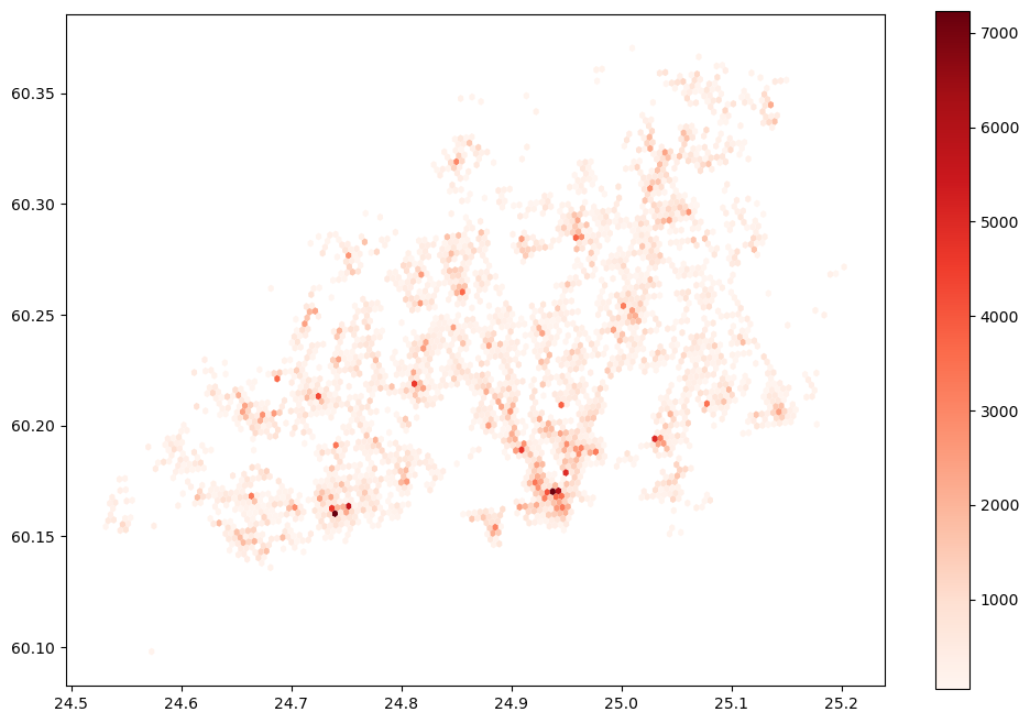
Now we can see the areas in Helsinki Region where the highest number of users are travelling to.

Exercise

Modify the above codes and produce a similar map based on the origin hexagons. Are the patterns similar?

# Write your solution here
# You can add new cells below if you want

Create a simple flowmap

Take a copy of the OD-data:

flows = data.copy()

Next, we will create a LineString object out of the origin and destination points:

from shapely import LineString

# Names of the hex columns
orig_hex = "origin_code_level_9"
dest_hex = "destination_code_level_9"

# Extract the Hexagon centroids for origins and destinations
flows["origin_geom"] = flows[orig_hex].apply(lambda x: Point(list(h3.h3_to_geo(str(x)))[::-1]))
flows["destination_geom"] = flows[dest_hex].apply(lambda x: Point(list(h3.h3_to_geo(str(x)))[::-1]))

# Create a LineString geometry out of the points
flows["line_geom"] = flows.apply(lambda x: LineString([x["origin_geom"], x["destination_geom"]]), axis=1)

Create a GeoDataFrame using the line geometry as input:

flows = gpd.GeoDataFrame(flows, geometry="line_geom", crs="epsg:4326")
flows.head(2)

	destination_code_level_9	origin_code_level_9	NUMBER_OF_USERS	DWELL_TIME	EXTRAPOLATED_NUMBER_OF_USERS	NUMBER_OF_SIGNALS	EXTRAPOLATED_NUMBER_OF_SIGNALS	PROPORTION_OF_USERS	NAMEFIN	geometry	origin_geom	destination_geom	line_geom
0	890899695b3ffff	89089961267ffff	0.666667	5.487959	92.888889	7.444444	935.555556	5.026455	Helsinki	POLYGON ((24.71888 60.16059, 24.72156 60.15990...	POINT (24.643168607702737 60.23880366998905)	POINT (24.72132081962259 60.161602839010435)	LINESTRING (24.64317 60.23880, 24.72132 60.16160)
1	8908996800bffff	89089968003ffff	3.666667	3.687860	362.555556	5.222222	509.666667	9.801587	Helsinki	POLYGON ((24.72557 60.18673, 24.72825 60.18605...	POINT (24.725095460617776 60.19013190739788)	POINT (24.72801569739153 60.18774882622088)	LINESTRING (24.72510 60.19013, 24.72802 60.18775)

Now we can make a simple plot showing the origin destination flows:

column = "EXTRAPOLATED_NUMBER_OF_USERS"
flows.plot(column=column, cmap="Reds", linewidth=flows[column]/1000, alpha=0.5, figsize=(12,12))

<Axes: >

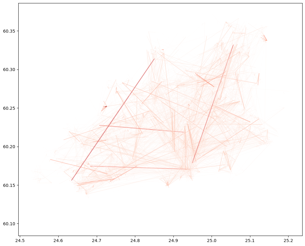
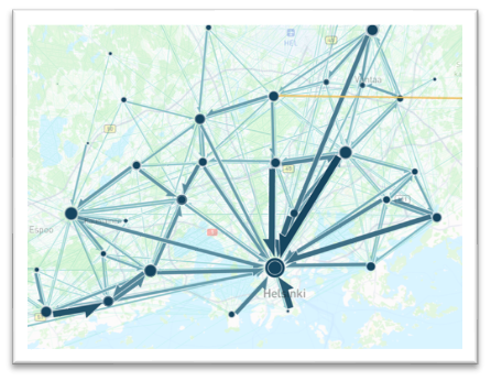
The map shows all the OD-flows in the region using Euclidian lines. The darker the color and the thicker the line, the more people have been travelling between these locations.

If you want to make a better looking map out of the flows, you can use e.g. FlowmapBlue or lonboard which enable you to create nice interactive maps out of the flows.

Retrieving POI data from online resources

In sustainable mobility studies, it is very typical that you want to understand how people can access specific opportunities (POIs) like education/schools, health services, and jobs. Naturally for being able to do these kind of analyses, you need to know where the services are located. Luckily, retrieving data about locations of services is quite easy in Python using libraries, such as osmnx or overturemaps. OSMnx allows you to retrieve any data that is stored in OpenStreetMap database on a global level, and overturemaps allows to do the same from Overture Maps Foundation’s database which is maintained by big tech companies, such as Amazon, Meta, Microsoft and TomTom.

The Overture Maps data has a higher quality compared to OSM especially for POIs which are constantly changing due to businesses emerging and closing down, as well as changing their locations. Hence, regular updates are needed. The large tech-companies are doing these updates on a regular basis (part of their business) whereas the OSM data is updated by volunteers who contribute to the OSM. For this reason, OSM tend to be slightly outdated and hence of poorer quality.

In the following, we show how you can retrieve OvertureMaps data using Python. Let’s start by finding the boundaries for the area that we are interested in using osmnx:

import osmnx as ox
import overturemaps
import shapely
import geopandas as gpd

# Area of Interest (the cities covering the Helsinki Region)
query = ["Helsinki", "Espoo", "Vantaa", "Kauniainen"]

# Find the boundaries for given areas of interest
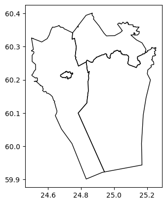
admin_area = ox.geocode_to_gdf(query)
admin_area.plot(facecolor="None")

<Axes: >

Now we have the boundaries for our area of interest. In the following, we will:

• Extract the bounding box rectangle of our area of interest

• Fetch the overture maps data from the area

• Convert the WKB (Well Known Binary) formatted geometries into normal shapely objects

• Create a GeoDataFrame out of the results that we can use for analysis and mapping

# Fetch the bounding box of the area 
bbox = admin_area.total_bounds.tolist()

# Fetch the data from overturemaps
table = overturemaps.record_batch_reader("place", bbox).read_all()

# Merge all chunks
table = table.combine_chunks()

# Convert Arrow Table into a DataFrame
df = table.to_pandas()

# Convert geometries from WKB format to normal geometries
df["geometry"] = shapely.from_wkb(df["geometry"])

# Create a GeoDataFrame out of the results
gdf = gpd.GeoDataFrame(df, crs="epsg:4326")
gdf.head()

	id	geometry	bbox	version	update_time	sources	names	categories	confidence	websites	socials	emails	phones	brand	addresses
0	08f089bb740ac48503784c44c5b8b3a2	POINT (24.51725 60.01297)	{'xmin': 24.51724624633789, 'xmax': 24.5172500...	0	2024-05-10T00:00:00.000Z	[{'property': '', 'dataset': 'meta', 'record_i...	{'primary': 'Bussarna', 'common': None, 'rules...	{'main': 'landmark_and_historical_building', '...	0.545360	None	[https://www.facebook.com/1308657845815075]	None	None	None	[{'freeform': None, 'locality': 'Kirkkonummi',...
1	08f089bb74b163930370d7806b3cc3af	POINT (24.50711 60.02024)	{'xmin': 24.507104873657227, 'xmax': 24.507108...	0	2024-05-10T00:00:00.000Z	[{'property': '', 'dataset': 'msft', 'record_i...	{'primary': 'Villa Vitsand', 'common': None, '...	{'main': 'venue_and_event_space', 'alternate':...	0.895433	[https://www.villavitsand.com/]	None	None	[0405799353]	None	[{'freeform': 'Klinthällantie 132', 'locality'...
2	08f089bb75cf63aa03cbc99ec04cdbe1	POINT (24.52478 60.02699)	{'xmin': 24.5247745513916, 'xmax': 24.52477836...	0	2024-05-10T00:00:00.000Z	[{'property': '', 'dataset': 'meta', 'record_i...	{'primary': 'Villa Hummerheim', 'common': None...	{'main': 'holiday_rental_home', 'alternate': [...	0.667112	[http://www.hummeripojat.fi/villa/villa_index....	[https://www.facebook.com/178985162147288]	None	None	None	[{'freeform': None, 'locality': None, 'postcod...
3	08f089bb7080e7190355975594d33372	POINT (24.53942 60.01895)	{'xmin': 24.539419174194336, 'xmax': 24.539422...	0	2024-05-10T00:00:00.000Z	[{'property': '', 'dataset': 'meta', 'record_i...	{'primary': 'Mössö', 'common': None, 'rules': ...	None	0.318976	None	[https://www.facebook.com/162053340528369]	None	None	None	[{'freeform': None, 'locality': None, 'postcod...
4	08f089bb70c55c41034b335ac6162349	POINT (24.54379 60.01303)	{'xmin': 24.543787002563477, 'xmax': 24.543790...	0	2024-05-10T00:00:00.000Z	[{'property': '', 'dataset': 'meta', 'record_i...	{'primary': 'Bötesören', 'common': None, 'rule...	{'main': 'landmark_and_historical_building', '...	0.667112	None	[https://www.facebook.com/1112597408814264]	None	None	None	[{'freeform': None, 'locality': 'Kirkkonummi',...

From this table we can see that the table contains a lot of information, such as:

• the categories which tells us what kind of POI the given feature is (e.g. a park, hospital, library, etc.)

• the confidence of the existence of the place which is a number between 0 and 1. 0 means that we’re sure that the place doesn’t exist (anymore). 1 means that we’re sure that the place exists.

• the website for the given POI

• the addresses for the place (locality, street address, etc.)

For analytical purposes, the most interesting attribute here is the categories which we can use to understand what kind of POIs we have at hand. This attribute is also useful because we can use it to filter specific types of services from the data (e.g. schools, hospitals). The categories include the main category identified for the POI as well, as alternative categories because a specific POI can belong to multiple categories at once.

In our case, we are now only interested in the main category of the POI. Hence, we will extract the main category from the dictionary and store it into a column main_category:

# Extract the main category from the data
gdf["main_category"] = gdf.categories.apply(lambda row: None if row is None else row["main"])
gdf.main_category.head()

0    landmark_and_historical_building
1               venue_and_event_space
2                 holiday_rental_home
3                                None
4    landmark_and_historical_building
Name: main_category, dtype: object

Now we have identified the main category and we can plot all the POIs on a map where the different colors indicate a specific category:

# Plot all POIs
gdf.plot(column="main_category", markersize=1.5, figsize=(12,12))

<Axes: >

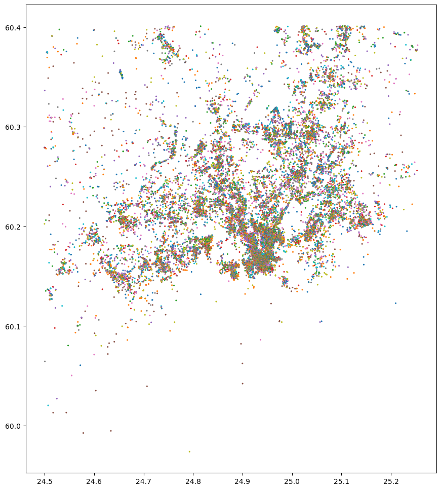
As we can see, there are thousands of POIs present in the data. In the following, we can count which categories are the most common ones in our data:

# Check how many POIs exist per category
gdf["main_category"].value_counts()

main_category
beauty_salon                        1682
community_services_non_profits      1208
professional_services               1191
park                                 924
landmark_and_historical_building     784
                                    ... 
football_stadium                       1
portuguese_restaurant                  1
african_restaurant                     1
cleaning_products_supplier             1
specialty_foods                        1
Name: count, Length: 963, dtype: int64

# To check all available categories, uncomment and run this
# gdf["main_category"].unique()

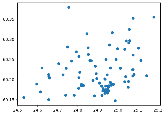
Finally, we can filter the data for specific categories that might be interesting for us. In the following, we filter data for libraries, hospitals and supermarkets that we can use later in our analyses:

# Select only specific services
libraries = gdf.loc[gdf["main_category"] == "library"].copy()
hospitals = gdf.loc[gdf["main_category"] == "hospital"].copy()
supermarkets = gdf.loc[gdf["main_category"] == "supermarket"].copy()
high_schools = gdf.loc[gdf["main_category"] == "high_school"].copy()

Now we have stored specific services into separate GeoDataFrames and we can plot them to see how they are distributed in the Helsinki Region:

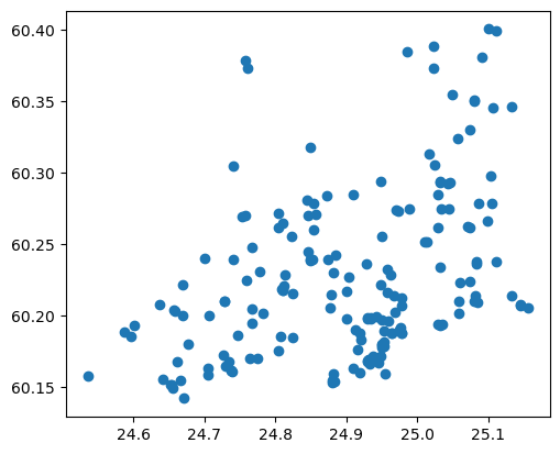
libraries.plot()

<Axes: >

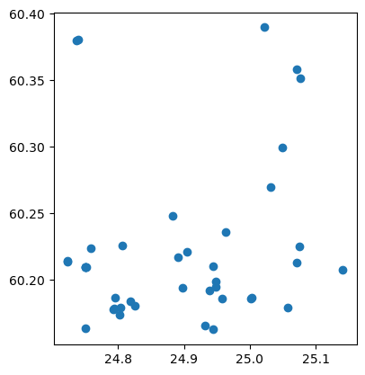
hospitals.plot()

<Axes: >

supermarkets.plot()

<Axes: >

high_schools.plot()

<Axes: >

Pre-calculated datasets

For this workshop, we have prepared various datasets that are stored into workshop_data folder. The folder pre-calculated matrices for car and public transport including information about:

• How many users travel between specific places (based on mobile phone data)

  • Column: EXTRAPOLATED_NUMBER_OF_USERS

• The travel time for travelling between these locations by a given transport mode

  • Column: Car_Travel_Time_minutes, and

  • Column: PT_Travel_Time_minutes

• The GHG emissions for a single person travelling between these locations for a given transport mode

  • Column: Single_CarTrip_Co2, and

  • Column: Single_PT_Trip_Co2

• The total sum of emissions considering that all users would travel between specific places with a specific transport mode

  • Column: Agg_CarTrip_Co2, and

  • Column: Agg_PT_Trip_Co2

In the below, we demonstrate how the pre-calculated data looks like:

import pandas as pd

# File paths
car_fp = "prepared_datasets/matrices/Car_trips_Helsinki.csv"
pt_fp = "prepared_datasets/matrices/Transit_trips_Helsinki.csv"

# Read information about car trips
car_trips = pd.read_csv(car_fp)
car_trips.head()

	origin_code_level_9	destination_code_level_9	NUMBER_OF_USERS	DWELL_TIME	EXTRAPOLATED_NUMBER_OF_USERS	NUMBER_OF_SIGNALS	EXTRAPOLATED_NUMBER_OF_SIGNALS	PROPORTION_OF_USERS	NAMEFIN	Single_CarTrip_Co2	Agg_CarTrip_Co2	Car_Travel_Time_minutes
0	89089961267ffff	890899695b3ffff	0.67	5.49	92.89	7.44	935.56	5.03	Helsinki	2335.92	75943.41	13.00
1	89089968003ffff	8908996800bffff	3.67	3.69	362.56	5.22	509.67	9.80	Helsinki	66.06	8382.21	0.85
2	89089968003ffff	8908996800fffff	0.67	2.01	71.00	0.89	92.22	1.01	Helsinki	35.69	886.99	0.46
3	89089968003ffff	8908996801bffff	0.67	2.67	79.11	1.22	154.11	4.02	Helsinki	130.82	3622.38	1.68
4	89089968003ffff	89089968063ffff	2.00	3.96	235.67	2.56	287.89	4.08	Helsinki	210.07	17327.18	2.70

# Read information about transit trips
transit_trips = pd.read_csv(pt_fp)
transit_trips.head()

	origin_code_level_9	destination_code_level_9	NUMBER_OF_USERS	DWELL_TIME	EXTRAPOLATED_NUMBER_OF_USERS	NUMBER_OF_SIGNALS	EXTRAPOLATED_NUMBER_OF_SIGNALS	PROPORTION_OF_USERS	NAMEFIN	Single_PT_Trip_Co2	Agg_PT_Trip_Co2	PT_Travel_Time_minutes
0	89089968bdbffff	890899612cbffff	1.22	2.11	115.78	4.33	409.44	5.03	Helsinki	427.37	11380.43	76.0
1	89089969503ffff	890899612cbffff	0.78	2.35	84.22	2.44	254.56	5.29	Helsinki	624.52	12097.62	76.0
2	8908996950bffff	890899612cbffff	0.67	2.17	62.00	1.67	154.78	1.10	Helsinki	514.48	7336.53	76.0
3	890899698c3ffff	890899612cbffff	0.89	5.21	90.44	3.56	354.33	12.70	Helsinki	872.00	18139.58	76.0
4	8908996800fffff	89089968003ffff	1.44	3.27	181.22	1.67	202.44	7.46	Helsinki	23.37	973.94	5.0

These matrices cover the data for the whole Helsinki Region where human activity has been observed based on mobile phone data during April-May 2023. You can combine this data e.g. with the OvertureMaps POI data to understand how people can travel to specific services and how many people on average travel to these given locations.

import geopandas 

# Read POI data
libraries = gpd.read_file("prepared_datasets/POIs/Helsinki_libraries.gpkg")
libraries.head()

	id	bbox	version	update_time	sources	names	categories	confidence	websites	socials	emails	phones	brand	addresses	main_category	geometry
0	08f089979c540d6e03884387347f4c9e	{'xmin': 24.531015396118164, 'xmax': 24.531019...	0	2024-05-10T00:00:00.000Z	[{'property': '', 'dataset': 'meta', 'record_i...	{'primary': 'Masala Library', 'common': None, ...	{'main': 'library', 'alternate': array(['cafe'...	0.959385	['http://itfmasala.fi']	['https://www.facebook.com/509593566224338']	None	['+358929672137']	None	[{'freeform': 'Sundsbergintie 1', 'locality': ...	library	POINT (24.53102 60.15436)
1	08f08997992ecaa9030b2bb0a94a4d62	{'xmin': 24.59498405456543, 'xmax': 24.5949878...	0	2024-05-10T00:00:00.000Z	[{'property': '', 'dataset': 'meta', 'record_i...	{'primary': 'Kauklahti Library', 'common': Non...	{'main': 'library', 'alternate': array(['publi...	0.959385	['http://www.helmet.fi/kauklahdenkirjasto']	['https://www.facebook.com/188329867875289']	None	['+358981653778']	None	[{'freeform': 'Hansakallio 2', 'locality': 'Es...	library	POINT (24.59498 60.18805)
2	08f08996b0118b9d03d23d77bd85d6fe	{'xmin': 24.655099868774414, 'xmax': 24.655103...	0	2024-05-10T00:00:00.000Z	[{'property': '', 'dataset': 'meta', 'record_i...	{'primary': 'Lippulaiva Library', 'common': No...	{'main': 'library', 'alternate': array(['publi...	0.959385	['https://helmet.finna.fi/organisationinfo/hom...	['https://www.facebook.com/101640745094450']	None	['+358981635097']	None	[{'freeform': 'Espoonlahdenkatu 8', 'locality'...	library	POINT (24.65510 60.14934)
3	08f089979b28dbb6037ca222777113bd	{'xmin': 24.614763259887695, 'xmax': 24.614767...	0	2024-05-10T00:00:00.000Z	[{'property': '', 'dataset': 'meta', 'record_i...	{'primary': 'Saunalahti Library', 'common': No...	{'main': 'library', 'alternate': array(['publi...	0.959385	['http://www.helmet.fi/saunalahdenkirjasto']	['https://www.facebook.com/246785858757196']	None	['+358981684645']	None	[{'freeform': 'Brinkinmäentie 1', 'locality': ...	library	POINT (24.61477 60.16872)
4	08f08996a389c9ae032ca429e8d1c7fc	{'xmin': 24.65976905822754, 'xmax': 24.6597728...	0	2024-05-10T00:00:00.000Z	[{'property': '', 'dataset': 'meta', 'record_i...	{'primary': 'Espoon Kirjastoautot', 'common': ...	{'main': 'library', 'alternate': array(['arts_...	0.363008	['https://helmet.finna.fi/content/kirjastoauto...	['https://www.facebook.com/28567010728']	None	['+358981657619']	None	[{'freeform': 'Valakuja 10a', 'locality': 'Esp...	library	POINT (24.65977 60.20299)

# Read Hexagons
hexagons = gpd.read_file("prepared_datasets/H3/h3_polygons_Helsinki.gpkg")
hexagons.head()

	ID	geometry
0	89089961267ffff	POLYGON ((24.64072 60.23779, 24.64341 60.23711...
1	89089968003ffff	POLYGON ((24.72265 60.18912, 24.72533 60.18843...
2	8908996800fffff	POLYGON ((24.72778 60.18945, 24.73046 60.18876...
3	8908996801bffff	POLYGON ((24.72044 60.18640, 24.72312 60.18572...
4	89089968063ffff	POLYGON ((24.73583 60.18740, 24.73851 60.18671...

# Find the hexagons under which the libraries belong to
library_hex = libraries.sjoin(hexagons, predicate="within")
library_hex.head()

	id	bbox	version	update_time	sources	names	categories	confidence	websites	socials	emails	phones	brand	addresses	main_category	geometry	index_right	ID
0	08f089979c540d6e03884387347f4c9e	{'xmin': 24.531015396118164, 'xmax': 24.531019...	0	2024-05-10T00:00:00.000Z	[{'property': '', 'dataset': 'meta', 'record_i...	{'primary': 'Masala Library', 'common': None, ...	{'main': 'library', 'alternate': array(['cafe'...	0.959385	['http://itfmasala.fi']	['https://www.facebook.com/509593566224338']	None	['+358929672137']	None	[{'freeform': 'Sundsbergintie 1', 'locality': ...	library	POINT (24.53102 60.15436)	2534	89089979c57ffff
2	08f08996b0118b9d03d23d77bd85d6fe	{'xmin': 24.655099868774414, 'xmax': 24.655103...	0	2024-05-10T00:00:00.000Z	[{'property': '', 'dataset': 'meta', 'record_i...	{'primary': 'Lippulaiva Library', 'common': No...	{'main': 'library', 'alternate': array(['publi...	0.959385	['https://helmet.finna.fi/organisationinfo/hom...	['https://www.facebook.com/101640745094450']	None	['+358981635097']	None	[{'freeform': 'Espoonlahdenkatu 8', 'locality'...	library	POINT (24.65510 60.14934)	2082	8908996b013ffff
3	08f089979b28dbb6037ca222777113bd	{'xmin': 24.614763259887695, 'xmax': 24.614767...	0	2024-05-10T00:00:00.000Z	[{'property': '', 'dataset': 'meta', 'record_i...	{'primary': 'Saunalahti Library', 'common': No...	{'main': 'library', 'alternate': array(['publi...	0.959385	['http://www.helmet.fi/saunalahdenkirjasto']	['https://www.facebook.com/246785858757196']	None	['+358981684645']	None	[{'freeform': 'Brinkinmäentie 1', 'locality': ...	library	POINT (24.61477 60.16872)	799	89089979b2bffff
4	08f08996a389c9ae032ca429e8d1c7fc	{'xmin': 24.65976905822754, 'xmax': 24.6597728...	0	2024-05-10T00:00:00.000Z	[{'property': '', 'dataset': 'meta', 'record_i...	{'primary': 'Espoon Kirjastoautot', 'common': ...	{'main': 'library', 'alternate': array(['arts_...	0.363008	['https://helmet.finna.fi/content/kirjastoauto...	['https://www.facebook.com/28567010728']	None	['+358981657619']	None	[{'freeform': 'Valakuja 10a', 'locality': 'Esp...	library	POINT (24.65977 60.20299)	401	8908996a38bffff
5	08f08996a3882ae403d03f3c59c781f0	{'xmin': 24.65888023376465, 'xmax': 24.6588840...	0	2024-05-10T00:00:00.000Z	[{'property': '', 'dataset': 'meta', 'record_i...	{'primary': 'Entressen kirjasto', 'common': No...	{'main': 'library', 'alternate': array(['publi...	0.959385	['http://www.helmet.fi/entressenkirjasto']	['https://www.facebook.com/53625091742']	None	['+358981653776']	None	[{'freeform': 'Siltakatu 11', 'locality': 'Esp...	library	POINT (24.65888 60.20364)	401	8908996a38bffff

# Find all trips by car and associated mobility data to these libraries
library_trips = car_trips.merge(library_hex, 
                                left_on="destination_code_level_9",
                                right_on="ID")

library_trips.columns                              

Index(['origin_code_level_9', 'destination_code_level_9', 'NUMBER_OF_USERS',
       'DWELL_TIME', 'EXTRAPOLATED_NUMBER_OF_USERS', 'NUMBER_OF_SIGNALS',
       'EXTRAPOLATED_NUMBER_OF_SIGNALS', 'PROPORTION_OF_USERS', 'NAMEFIN',
       'Single_CarTrip_Co2', 'Agg_CarTrip_Co2', 'Car_Travel_Time_minutes',
       'id', 'bbox', 'version', 'update_time', 'sources', 'names',
       'categories', 'confidence', 'websites', 'socials', 'emails', 'phones',
       'brand', 'addresses', 'main_category', 'geometry', 'index_right', 'ID'],
      dtype='object')

# How many OD-pairs there are?
library_trips.shape

(636, 30)

# First rows (note: Not all columns are visible)
library_trips.head(5)

	origin_code_level_9	destination_code_level_9	NUMBER_OF_USERS	DWELL_TIME	EXTRAPOLATED_NUMBER_OF_USERS	NUMBER_OF_SIGNALS	EXTRAPOLATED_NUMBER_OF_SIGNALS	PROPORTION_OF_USERS	NAMEFIN	Single_CarTrip_Co2	...	websites	socials	emails	phones	brand	addresses	main_category	geometry	index_right	ID
0	89089968063ffff	891126d338bffff	0.78	2.35	75.56	1.67	164.89	2.78	Helsinki	2288.54	...	None	['https://www.facebook.com/327890987935991']	None	None	None	[{'freeform': None, 'locality': 'Helsinki', 'p...	library	POINT (24.93738 60.16792)	1813	891126d338bffff
1	8908996836fffff	891126d338bffff	1.78	2.20	211.44	3.11	359.33	3.26	Helsinki	1828.60	...	None	['https://www.facebook.com/327890987935991']	None	None	None	[{'freeform': None, 'locality': 'Helsinki', 'p...	library	POINT (24.93738 60.16792)	1813	891126d338bffff
2	890899691afffff	891126d338bffff	0.78	3.22	87.44	1.89	206.33	1.93	Helsinki	1611.93	...	None	['https://www.facebook.com/327890987935991']	None	None	None	[{'freeform': None, 'locality': 'Helsinki', 'p...	library	POINT (24.93738 60.16792)	1813	891126d338bffff
3	891126d0c03ffff	891126d338bffff	1.00	5.95	131.11	5.56	633.11	2.94	Helsinki	1876.20	...	None	['https://www.facebook.com/327890987935991']	None	None	None	[{'freeform': None, 'locality': 'Helsinki', 'p...	library	POINT (24.93738 60.16792)	1813	891126d338bffff
4	891126d1e37ffff	891126d338bffff	0.56	2.14	64.33	1.33	136.56	1.81	Helsinki	1538.29	...	None	['https://www.facebook.com/327890987935991']	None	None	None	[{'freeform': None, 'locality': 'Helsinki', 'p...	library	POINT (24.93738 60.16792)	1813	891126d338bffff

5 rows × 30 columns

# Generate flows to the libraries
# -------------------------------

from shapely import Point, LineString

# Names of the hex columns
orig_hex = "origin_code_level_9"
dest_hex = "destination_code_level_9"

library_flows = library_trips.copy()

# Extract the Hexagon centroids for origins and destinations
library_flows["origin_geom"] = library_flows[orig_hex].apply(lambda x: Point(list(h3.h3_to_geo(str(x)))[::-1]))
library_flows["destination_geom"] = library_flows[dest_hex].apply(lambda x: Point(list(h3.h3_to_geo(str(x)))[::-1]))

# Create a LineString geometry out of the points
library_flows["line_geom"] = library_flows.apply(lambda x: LineString([x["origin_geom"], x["destination_geom"]]), axis=1)

# Create a GeoDataFrame
library_flows = gpd.GeoDataFrame(library_flows, geometry="line_geom", crs="epsg:4326")

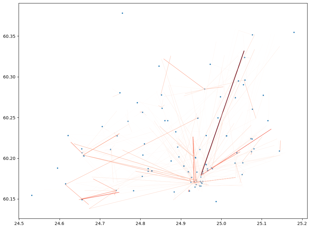
# Visualize the flows to hexagons where libraries are located
column = "EXTRAPOLATED_NUMBER_OF_USERS"

ax = library_flows.plot(column=column, cmap="Reds", linewidth=library_flows[column]/1000, alpha=0.9, figsize=(12,12))
ax = libraries.plot(ax=ax, markersize=4)

In a similar manner, you can combine the data and investigate the mobilities and associated travel times and GHG emissions to other Points of Interests, which are provided for you.

In case you are interested how these datasets were produced, take a look on:

• Tutorial 1: Travel time and carbon emission quantification for car-based trips

• Tutorial 2: Travel time and carbon emission quantification for transit based trips

Also, in case you would be interested to know how to calculate travel time matrices for larger areas, you can take a look on following tutorial (out of scope for this workshop):

• Spatial Accessibility Modelling with r5py